Force Platform - Center of Pressure Estimation

Difficulty Level:

Posture is an important indication of the health of the muscles involved in it. Specifically, there are specialised muscles involved in maintaining a correct posture, being it standing, sitting or laying down, which should be involuntarily activated. When those muscles are not well adjusted, other muscles need to compensate, resulting in possible back pain or inflammation.

Bad posture can be caused by poor work environment, incorrect working posture, unhealthy sitting and standing habits, stress, obesity, etc. So, identifying bad posture is only the first step to solve it, because it is the cause that should be corrected.

There are multiple ways to assess posture. One of them may be by the analysis of the center of pressure that gives an indication regarding the posture while standing .

The current Jupyter Notebook will demonstrate how to use a force platform in order to calculate the center of pressure.

1 - Import required packages

These packages will facilitate our job, as they provide a set of functions that we would need to implement otherwise.

# biosignalsnotebooks project own package.
import biosignalsnotebooks as bsnb

# Powerful scientific package for array operations.
from numpy import array

2 - Load the Signal

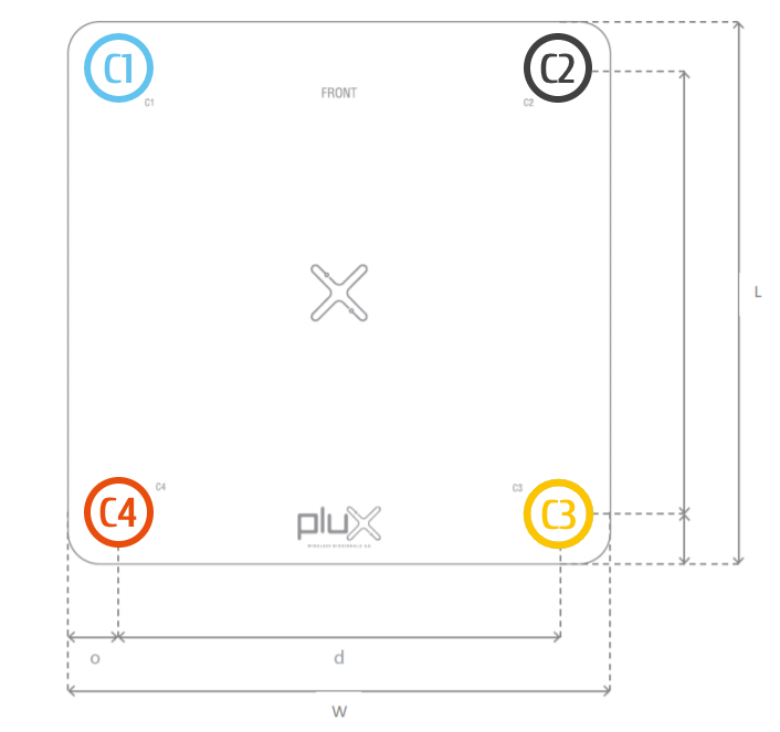
To calculate the center of pressure, we used a force platform.
The force platform is composed by 4 load cells that represent channels to our devices. Here, we will load the signals from the platform and from each channel.

path_to_file = "/signal_samples/loft_time_subject_1.h5"

# Load the data from the file
force_platform = bsnb.load(path_to_file)

# Identify the mac address of the device
force_platform_mac, _ = force_platform.keys()

# Get the signals acquired by the force_platform
force_platform_signals = force_platform[force_platform_mac]

The next step consists on getting the signal of each load cell and store it in a new list.

load_cells = []
for load_cell in force_platform_signals.keys():
    load_cells.append(force_platform_signals[load_cell])

3 - Raw Signal Conversion

The signals need to be converted to weight in order to be used ahead.

In order to convert those signals to weight, we need to specify every constant to be used on the conversion formula. Both the formula to convert the raw signal to weight and to calculate the center of pressure were taken from the Force Platform datasheet .

The V$_{FS}$ constants are specific for each load cell and are obtained by a calibration process (supplied during the purchase).

# Constant for load cell 1.
Vfs_1 = 2.00061
# Constant for load cell 2.
Vfs_2 = 2.00026
# Constant for load cell 3.
Vfs_3 = 2.00011
# Constant for load cell 4.
Vfs_4 = 2.00038

C = 406.831 # kg.mV/V

# Sampling rate used during the acquisition.
sr = 500 # Hz

# Resolution of the device.
resolution = 16 # bits

The next step consists in converting the raw signal samples ($ADC$) to weight. In order to do that, we will use the formula:

$ Weight = \dfrac{ADC \times C}{V_{FS}(2^{resolution} - 1)} $

We converted that formula to a Python function so that it is direct to calculate the weight applied for each load cell.
Note that $C$ is a constant common to all Load Cells and $V_{FS}$ is the previously mentioned calibration values specific of each Load Cell

def weight(ADC, Vfs, C, resolution):
    return array(ADC) * C / (Vfs * ( (2**resolution) - 1 ) )

Thus, we can apply the function for each load cell such as demonstrated on the following cell.

weight_1 = weight(load_cells[0], Vfs_1, C, resolution)
weight_2 = weight(load_cells[1], Vfs_2, C, resolution)
weight_3 = weight(load_cells[2], Vfs_3, C, resolution)
weight_4 = weight(load_cells[3], Vfs_4, C, resolution)

The next plots show the evolution in time of the weight applied in each load cell. We can see that if we sum them, we get an almost constant value around the true weight of the subject, so, the formula is applicable. Furthermore, there are changes on the force applied to each load cell, which means that the center of pressure moved during the acquisition, therefore, we should be able to see those movements on a plot of the position of the center of pressure .

sr = 500 # Hz
resolution = 16 # bits

load_cells = [weight_1, weight_2, weight_3, weight_4]
trimmed_load_cells = load_cells
for i in range(len(trimmed_load_cells)):
    t_i = 22
    t_f = 35
    trimmed_load_cells[i] = bsnb.smooth(load_cells[i][t_i*sr:t_f*sr], 20)

time = bsnb.generate_time(trimmed_load_cells[0], sr)
times = []
for i in range(len(trimmed_load_cells)):
    times.append(time)

bsnb.plot(times, trimmed_load_cells, grid_plot=True, grid_lines=2, grid_columns=2, x_axis_label='Time (s)', 
          y_axis_label='kgf', title=["Load Cell 1", "Load Cell 2", "Load Cell 3", "Load Cell 4"], line_dash='dotted')

weight_1, weight_2, weight_3, weight_4 = trimmed_load_cells.copy()

4 - Calculating the Center of Pressure

The final part of the process is to calculate the center of pressure.

There are two formulas we need to apply in order to calculate the center of pressure on the corresponding x and y axis relative to the center of the platform.

$ {Center\ of\ Pressure}_x = \dfrac{W}{2}\dfrac{C_2 + C_3 - C_1 - C_4}{C_1 + C_2 + C_3 + C_4} $

$ {Center\ of\ Pressure}_y = \dfrac{L}{2}\dfrac{C_2 + C_1 - C_3 - C_4}{C_1 + C_2 + C_3 + C_4} $

where $W$ and $L$ are specified in the datasheet of the force platform and represent the width and length and $C_1$, $C_2$, $C_3$ and $C_4$ represent the weight applied in each cell. Thus, we only need to specify these variables, such as in the next cell, and apply the formulas.

W = 450 # mm
L = 450 # mm
C1 = weight_1
C2 = weight_2
C3 = weight_3
C4 = weight_4

# Get the center of pressure on the x axis
center_of_pressure_x = (W/2)*(C2 + C3 - C1 - C4)/(C1 + C2 + C3 + C4)
# Get the center of pressure on the y axis
center_of_pressure_y = (L/2)*(C2 + C1 - C3 - C4)/(C1 + C2 + C3 + C4)

If we plot the center of pressure on the x axis as a function of the center of pressure on the y axis, we can see the movement of the overall center of pressure in relation to the force platform.

#%matplotlib notebook
%matplotlib inline
import matplotlib.pylab as plt
import seaborn as sns
sns.set()
sns.set_style("whitegrid", {"axes.facecolor": ".95", "grid.linestyle": ':'})
plt.figure(figsize=(7, 7))
plt.scatter(center_of_pressure_x, center_of_pressure_y, marker=r'.', linewidths=1, c="#009EE3")
plt.xlabel("x Axis")
plt.ylabel("y Axis")
plt.title("Center of Pressure")
plt.xlim(-225,  225)
plt.ylim(-225,  225)
#plt.subplots_adjust(left=0.3, right=0.7)
plt.show()

from IPython.display import display, HTML
js = """<script>
//document.getElementsByClassName("ui-dialog-titlebar")[0].parentElement.parentElement.style.textAlign = "center";
document.getElementsByClassName("output_png")[0].style.textAlign = "center";
</script>"""
display(HTML(js))

This signal could then be analysed by a specialist to extract information regarding the posture of the subject or an algorithm could be developed to extract features from the signal and automatically assess about the patient"s health.

With this notebook we saw how straightforward it is to calculate the center of pressure using the force platform given the information available in the sensor"s datasheet.

We hope that you have enjoyed this guide. biosignalsnotebooks is an environment in continuous expansion, so don"t stop your journey and learn more with the remaining Notebooks !

☌ Project Presentation
☌ GitHub Repository
☌ How to install biosignalsnotebooks Python package ?
☌ Signal Library

☌ Notebook Categories
☌ Notebooks by Difficulty
☌ Notebooks by Signal Type
☌ Notebooks by Tag

from biosignalsnotebooks.__notebook_support__ import css_style_apply
css_style_apply()

.................... CSS Style Applied to Jupyter Notebook .........................