|
|
|
|
|
|
|
|
|
Calculate Time of Flight |
Jumping is an
important task
![]() to assess the physical health of individuals, particularly in athletes. There are many features that may be studied in each jump, such as the time of flight or loft. This particular feature may indicate the muscle strength of the lower body in relation to the weight of the athlete and can be used as an assessment for the training plan of the said athlete.
to assess the physical health of individuals, particularly in athletes. There are many features that may be studied in each jump, such as the time of flight or loft. This particular feature may indicate the muscle strength of the lower body in relation to the weight of the athlete and can be used as an assessment for the training plan of the said athlete.
The current
Jupyter Notebook
focuses on the presentation of a method to extract the loft time using either an
acceleration signal
![]() or a
force signal
or a
force signal
![]() of different sensors.
of different sensors.
1 - Acquisition Procedure
In order to assess the loft time and extract the multiple features from the accelerometer and force platform, a replicable protocol should be defined.In this case, the accelerometer was taped to the lower back of the subject in order to be as close as possible to the center of mass. Thus, it is possible to track the exact accelerometry of the subject and have a higher degree of certainty regarding their movements.
Furthermore, the subjects jumped vertically on the force platform without any horizontal movement.
|
2 - Load Signals
In this section it will be shown how to load the signals using the biosignalsnotebooks Python package.2.1 - Import the required packages
# biosignalsnotebooks project own package.
import biosignalsnotebooks as bsnb

# Powerful scientific package for array operations.
from numpy import array, min, where, ptp, mean, sqrt, sum, diff, abs, any
2.2 - Load the signals
Given that the acquisitions involved two devices - the force platform and a biosignalsplux accelerometer - it will be necessary to load the signals from both of them. Fortunately, the signals are stored in a single file, therefore, we only need to load it once.After that, the signals of each device will be extracted from the file given the mac address .
# Define the path of the file that has the signals of each device
path_subject_1 = "/signal_samples/loft_time_subject_1.h5"

# Load the data from the file
data_1 = bsnb.load(path_subject_1)

# Identify the mac addresses of each device
force_platform_1, accelerometer_1 = data_1.keys()

# Get the signals acquired by the force_platform
force_platform_signals_1 = data_1[force_platform_1]

# Get the signals acquired by the accelerometer
accelerometer_signals_1 = data_1[accelerometer_1]

# Sampling frequency of the acquisitions
fs = 500 # Hz
Each device acquired a different number of channels, corresponding to different signals.
Specifically, the force platform acquired data using
four channels
, while the accelerometer acquired data on three channels corresponding to each tridimensional axis.
The next cell will show how to get the data from each device and from each channel of each device.
For that, the first subset will be dedicated to initiate different lists for different devices and different experiments. Then, it will be ensured the iteration over each channel of each device to store those signals in the corresponding list.
2.3 - Initialisation of lists that will store the physiological data contained inside the loaded file
# This is the list where we will store the signals from each channels of the force platform.
# It is initiated as an empty lists so we can append items to it.
force_platform_channels_1 = []

# And this is the list where we will store the signals from each direction of the accelerometer.
accelerometer_direction_1 = []
2.4 - Populate the initialised lists
This is the part where we get the signal from each channel and append it to the corresponding list.The syntax of the following code lines may be a bit odd at first sight, so we recommend you to read: https://realpython.com/iterate-through-dictionary-python/
Force Platform
# Basically, force_platform_signals_1.keys() is a structure that iterates over the channels of the force platform device.
for channel in force_platform_signals_1.keys():
    # First, we get the signal of the channel
    channel_signal_1 = force_platform_signals_1[channel]
    # Then append the signal to the list that will contain the signals.
    force_platform_channels_1.append(channel_signal_1)
Accelerometer
# Now we need to do the same for the accelerometer. Note that the code is very similar compared to the force platform.
for direction in accelerometer_signals_1.keys():
    direction_signal_1 = accelerometer_signals_1[direction]
    accelerometer_direction_1.append(direction_signal_1)
|
|
CHECKPOINT |
|
The next plots are intended to show the signals generated by the force platform.
Here, they were trimmed to show only the most relevant time segment for the current application, which is the jump, and it can clearly be seen that it has a remarkable shape: first the signals are stable, meaning that the subject is at rest. Then, when the subjects start to flex their legs, the signal increases, meaning that there is a rising force being applied to the platform.
The minimum force applied during the flex corresponds to the position of maximum flex of the legs, in which the force on the platform is reduced. Then, there is a significant increase of the signal that corresponds to the increasing force being applied as the legs start to stretch to lift the whole body. The next segment of the signal, corresponding of 0"s, is the time interval when the feet leave the platform and, so, there is no pressure on it. The next structure, composed of a peak and a valley corresponds to the landing part of the jump.
For the accelerometer, the signals are not as clear as the ones generated by the force platform, but may still be valid to assess the loft time.
Essentially, each axis should be observed to see the differences between the rest state and the jump. For example, on the x axis , it is visible an increase of the variance of the acceleration during the jump; in the y axis a similar structure, as the one seen in the force platform, can be identified; in the z axis the structure seems a mix of the x and y axis.
The problem with this analysis, is that it depends on the placement of the accelerometer, therefore, a detection algorithm should be able to do the analysis regardless of the said placement. In order to do that, it should be calculated the magnitude of the signal, which corresponds to the combination of the 3 axis to generate one signal that is equally influenced by each signal, as expressed in the next expression:
In the calculus of the squared value of each direction, the mean is subtracted and the minimum value of all axis should be added, in order to normalize the signals. This way, it is guaranteed that no axis has more influence than the rest due to a baseline acceleration, such as, gravity. It is also ensured that all signals are positive.
|
|
END OF CHECKPOINT |
|
2.5 - Calculation of magnitude signal from the 3D accelerometer
2.5.1 - Conversion of lists to an array format where entry to entry operations can be easily applicable
# These first lines will get each direction that are required to calculate the magnitude.
experiment_1_direction_x = array(accelerometer_direction_1[0])
experiment_1_direction_y = array(accelerometer_direction_1[1])
experiment_1_direction_z = array(accelerometer_direction_1[2])
2.5.2 - Normalization of the accelerometer data from the 3 available axes
# Now, we need to calculate the square of each normalised direction
experiment_1_direction_x_squared = experiment_1_direction_x - mean(experiment_1_direction_x) + min([accelerometer_direction_1])
experiment_1_direction_y_squared = experiment_1_direction_y - mean(experiment_1_direction_y) + min([accelerometer_direction_1])
experiment_1_direction_z_squared = experiment_1_direction_z - mean(experiment_1_direction_z) + min([accelerometer_direction_1])
2.5.3 - Determination of the accelerometer magnitude through the application of the previously presented equation of magnitude (and replicated below)
# The next step is to sum the square of each direction
sum_all_direction_squared_1 = experiment_1_direction_x_squared**2 + experiment_1_direction_y_squared**2 + experiment_1_direction_z_squared**2

# And finaly apply the square root
magnitude_1 = sqrt(sum_all_direction_squared_1)
On the magnitude signal, it can be seen the gathered influence of each axis that does not depend on the orientation of the sensor while acquiring data.
>>>>>> Subject 1
Specifically, on this first experiment/subject the flight time corresponds to a valley on the magnitude signal.
3 - Signal Analysis
Following the eye analysis and structures identification, we can start to computationally identify the structures that indicate the beginning and ending of the jump.Through the visual inspection of force platform and accelerometer signals, it can be seen that the flight time corresponds to a plateau, for this particular subject the plateau is negative.
The loft time corresponds to the time the subject is not touching the platform, which is identifiable as the plateau between the peaks that correspond to the jumping and landing.
In the case of this first experiment , the loft time is estimated to be 0.340 seconds (refer to the figures of the previous section).
In this section, it will be explained how to implement an algorithm that may be able to calculate loft times using the accelerometer signal.
Note: Of course, the 0.340 seconds reference value is an estimate, because when no force is being applied, the platform still has to go back to the baseline position, in which it still detects some force, creating a bias. One way to take that into consideration would be to increase the threshold that flags the "no force" state, when no force is being applied to the platform.
3.1 - Algorithm Description
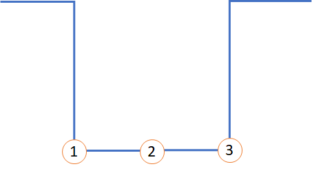
The algorithm is based on the structure of the plateau. The plateau, shown in the figure below will help us to analyse the general case.
|
Negative Plateau
Each specific point and all the structures around them will be analysed.
- On the left side of point number 1 there is a high negative slope, meaning that it has a high and negative derivative while on the right side the signal is constant, meaning the derivative is 0 or very low.
- On number 2 the condition is the same as on the previous case, which is that the signal is constant and, thus, the derivative must be 0 or very low.
- On the left of point number 3 the signal is constant and, therefore, the derivative is 0 or very low. On the right side of the point there is a high slope that rises the signal, meaning that the derivative is high and positive.
The next task consists on translating the previous description into code.
What should be taken into account is that when referring to
"very low"
or
"very high"
terms, it is necessary to specify thresholds that objectively define what those mean.
3.1.1 - Definition of thresholds and constants
First, the procedure will start with the definition of all the thresholds that the algorithm will need to apply. These values can be adapted to each individual application, but in this specific experiment they will be defined based on empirical observations. Specifically, based on our observations, both very low and very high threshold values will be the same and the same values will be used for the positive threshold.# Thresholds for the limiting points (1 and 3)
very_low_limiting_threshold = 100
very_high_limiting_threshold = 100
# Threshold for the point number 2
very_low_threshold = 700
# Threshold specifying that there are no jumps that take less than 0.1 seconds.
# The multiplication by the sampling rate is the conversion to the number of points in 0.1 seconds.
delta_t = 0.1*fs
Next, it will be necessary to iterate over the signal and apply the conditions of each of the three points. Given that our analysis is based on the signal
and
the derivative, we need to first calculate it. Moreover, a
low pass filter
![]() will be applied in order to reduce the noise and keep only the most relevant structures.
will be applied in order to reduce the noise and keep only the most relevant structures.
# Application of the low pass filter using a cut-off frequency of 10 Hz. The use_filtfilt argument states that
# the same filter is applied forward and backwards in order to reduce the artifacts the first filter may introduce.
filtered_magnitude_1 = bsnb.lowpass(magnitude_1, 10, fs=fs, use_filtfilt=True)

# Here we get the derivative of the signal of magnitude of the first experiment
derivative_magnitude_1 = diff(filtered_magnitude_1)
Now we have all the conditions to write the actual code that will look for each point. Some comments are available on the code in order to facilitate the explanation, so, beware of them while reading the code.
3.1.2 - Initialisation of variables
First, we will initialise the list where the limiting points will be stored. Specifically, it will be used one list to store the provisional points and another that will store the final points. The difference is that the final list will contain the points that meet all conditions to be considered a limiting point.# Here we initialise the list that will contain the provisional points limiting the plateau(s).
low_plateau = []
# Here we initialise the list that will contain the final points limiting the plateau(s).
low_final_plateau = []
Second, a flag, that will inform the algorithm what was the point that was last identified, will be initialised.
This is important because we should not look for consecutive left point or consecutive right points. The order should be always the same: we first find a left limiting point, then we find a right limiting point. Additionally, we can only start to look again for a left limiting point after both limiting points were found.
# This flag will be used to tell us if the algorithm has found a left limiting point, because it does not make sense to look for consecutive
# left limiting points if we have not found a right one.
low_flag = False
3.1.3 - Check which point meet the defined conditions
This is the tricky part. The next cell shows how we look for the provisional limiting points. Specifically, it iterates over the signal and checks if the conditions we set are met.
# Iterate over all points in the derivative except the first and last ones. This is because we will be looking for left and right points, and, so,
# we cannot look to the left of the first point and the right of the last point.
for point in range(1, len(derivative_magnitude_1)-1):

    # Get the point immediately at the left of the current one.
    left_point = derivative_magnitude_1[point-1]

    # Get the point immediately at the right of the current one.
    right_point = derivative_magnitude_1[point+1]

    # This says that only if the flag is false, meaning that no left limiting point was found, does the algorithm look for a left limiting point.
    # Else, it will look for a right limiting point.
    if not low_flag:
        # Definition of point number 1

        # If all the identified conditions verify, we store the point as a left limiting point.
        if abs(left_point) > very_high_limiting_threshold and  left_point < 0 and abs(right_point) < very_low_limiting_threshold:
            low_plateau.append(point)

            # The flag turns to true to specify that we have found a left limiting point.
            low_flag = True
    else:
        # Definition of point number 3
        # We check if the time threshold specified before is respected and only if it is does the algorithm look for a right limiting point.
        if point - low_plateau[-1] > delta_t:

            # If all the identified conditions verify, we store the point as a right limiting point.
            if abs(left_point) < very_low_limiting_threshold and abs(right_point) > very_high_limiting_threshold and right_point > 0:
                low_plateau.append(point)

                # Then we say that the flag is false so that new left limiting points can be found.
                low_flag = False
3.1.4 - Remove unpaired left points (avoiding incomplete intervals)
Given the provisional points, we should check if there is any left limiting point without a right correspondent. Due to the construction of the code, it can only happen if the last point is a left point and, so, we just need to see the state of the flag. If it is True, it means that the last point it found was a left one, and thus can be eliminated from the list.# If a left limiting point was found but not the right corresponding one, we should discard it.
if low_flag:
low_plateau.pop()
3.1.5 - Verification of which provisional points can be included in the final list of valid delimiting values for the start and end of the jump
Finally, we can check if the final condition is met. The final condition is that there is no point in between limiting points with a derivative higher than the threshold we defined. Only if that criteria is met are the points considered as true limiting points and are stored on the list containing the final points.# Only if we have more than two points do we check if they are suitable to be considered as limits of a plateau.
if len(low_plateau) >= 2:
# Here we will iterate over all points but in a pairwise condition, because a plateau is always limited by two points in our algorithm.
for point in range(0, len(low_plateau)-2, 2):
# [Definition of point number 2]
# If there are no point in between limiting points with a derivative higher than the threshold, then those are really limiting points and
# are stored in the final list.
if not any(derivative_magnitude_1[low_plateau[point]:low_plateau[point+1]] > very_low_threshold):
low_final_plateau.append(low_plateau[point])
low_final_plateau.append(low_plateau[point+1])
Now, it is necessary to check if the algorithm worked as expected and compare the estimated time using this algorithm to the time we calculated using the force platform signals.
The plot below shows the points the algorithm found as the vertical lines and we see that the plateau was found.
|
|
SUPPLEMENT |
|
The previously presented algorithm is truly useful to estimate the loft time using accelerometry sensors, however, all criteria were defined taking into consideration the premise that the plateau is negative.
In order to make the algorithm specification more generic, the opposite case (positive plateau) should be considered, being the following steps dedicated to provide an explanation about the needed steps.
S1 - Steps contained in section 2.x of the main text should be replicated
Those steps are dedicated to load the signal and prepare data to be applicable to the detection algorithm. They are not explicitly presented here but you can access it in the extended version of the Notebook, by clicking on the PROGRAM button available on the header.>>>>>> Subject 2
|
Force Platform
In the case of this second experiment , the loft time is estimated to be 0.404 seconds .
Accelerometer
S2 - Algorithm Description
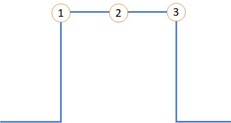
The plateaus, shown in the figure below will help us to analyse the general case.
|
Positive Plateau
The analysis is very similar to the negative plateau with some nuances, which are what makes the difference.
- On the left side of point number 1 there is a high positive slope, meaning that it has a high and positive derivative while on the right side the signal is constant, meaning the derivative is 0 or very low.
- On number 2 there is only one condition, which is that the signal is always constant, so, the derivative is 0 or very low.
- On the left of point number 3 the signal is constant and, therefore, the derivative is 0 or very low. On the right side of the point there is a high slope and the signal decreases, meaning that the derivative is high and negative.
S2.1 - Filtering the signal
# Application of the low pass filter using a cut-off frequency of 10 Hz. The use_filtfilt argument states that
# the same filter is applied forward and backwards in order to reduce the noise the first filter may introduce.
filtered_magnitude_2 = bsnb.lowpass(magnitude_2, 10, fs=fs, use_filtfilt=True)

# Here we get the derivative of the signal of magnitude of the second experiment
derivative_magnitude_2 = diff(filtered_magnitude_2)
S2.2 - Application of detection conditions
Now we have everything we need to apply a very similar algorithm as the one used to detect the negative plateau. Notice that the major difference on the next code cell are the conditions used to detect the limiting points. We also changed the names of the variables in order to clearly distinguish them from the previous case. In this case we do not explain each step of the algorithm because the steps are the same as on the previous case.# Here we initialise the list that will contain the provisional points limiting the plateau(s).
high_plateau = []
# Here we initialise the list that will contain the final points limiting the plateau(s).
high_final_plateau = []
# This flag will be used to tell us if the algorithm has found a left limiting point, because it does not make sense to look for consecutive
# left limiting points if we have not found a right one.
high_flag = False
###############################################################################
######################## Finding the limiting points ########################
###############################################################################
# Iterate over all points in the derivative except the first and last ones. This is because we will be looking for left and right points, and, so,
# we cannot look to the left of the first point and the right of the last point.
for point in range(1, len(derivative_magnitude_2)-1):
# Get the point immediately at the left of the current one.
left_point = derivative_magnitude_2[point-1]
# Get the point immediately at the right of the current one.
right_point = derivative_magnitude_2[point+1]
# This says that only if the flag is false, meaning that no left limiting point was found, does the algorithm look for a left limiting point.
# Else, if it found a left limiting point, it will look for a right limiting point.
if not high_flag:
# Definition of point number 1
# If all the identified conditions verify, we store the point as a left limiting point.
if abs(left_point) > very_high_limiting_threshold and left_point > 0 and abs(right_point) < very_low_limiting_threshold:
high_plateau.append(point)
# The flag turns to true to specify that we have found a left limiting point.
high_flag = True
else:
# Definition of point number 3
# We check if the time threshold specified before is respected and only if it is does the algorithm look for a right limiting point.
if point - high_plateau[-1] > delta_t:
# If all the identified conditions verify, we store the point as a right limiting point.
if abs(left_point) < very_low_limiting_threshold and abs(right_point) > very_high_limiting_threshold and right_point < 0:
high_plateau.append(point)
# Then we say that the flag is false so that new left limiting points can be found.
high_flag = False
# If a left limiting point was found but not the right corresponding one, we should discard it.
if high_flag:
high_plateau.pop()
# Only if we have more than two points do we check if they are suitable to be considered as limits of a plateau.
if len(high_plateau) >= 2:

    # Here we will iterate over all points but in a pairwise condition, because a plateau is always limited by two points in our algorithm.
    for point in range(0, len(high_plateau)-2, 2):

        # Definition of point number 2

        # If there are no point in between limiting points with a derivative higher than the threshold, then those are really limiting points and
        # are stored in the final list.
        if not any(derivative_magnitude_2[high_plateau[point]:high_plateau[point+1]] > very_low_threshold):
            high_final_plateau.append(high_plateau[point])
            high_final_plateau.append(high_plateau[point+1])
Once again, we will check if the algorithm worked as expected and compare the estimated time using this algorithm to the time we calculated using the force platform signals. The plot below shows the points the algorithm found as the vertical lines and we see that the plateau was found.
We saw that accelerometer signals are not the most reliable to calculate the time of flight of a jumping person, but can still be used if a proper post-analysis is applied. Specifically, the signals should be analysed before starting the development of any algorithm, in order to try to identify the most distinguishable structures that correspond to the actions we look for.
Furthermore, accelerometers may be a well suited solution for applications where high precision is not a concern, because they may not be as precise as other specific sensors. The big advantage of accelerometers is that they can be used outside of the laboratory and in a wide range of applications.
We hope that you have enjoyed this guide.
biosignalsnotebooks
is an environment in continuous expansion, so don"t stop your journey and learn more with the remaining
Notebooks
![]() !
!