|
|
|
|
|
|
|
|
|
Rock, Paper or Scissor Game - Train and Classify [Volume 1] |
| Tags | train_and_classify☁machine-learning☁acquisition |
Machine Learning
is a very suggestive term to define this scientific area and the "result" of their algorithms.
"Machine Learning grew out of the quest for artificial intelligence"
![]() , which inspires many people in building a totally new world with endless possibilities.
, which inspires many people in building a totally new world with endless possibilities.
In fact, only the idea of creating an intelligent system (even artificially) is both amazing and scaring, like all the ideas and discoveries which allowed to overcome a barrier that was previously considered as immutable.
In a very generic and simplistic way,
Machine Learning
includes the tools (algorithms) that computers can use in order to learn and acquire knowledge based on examples. The process that causes the acquisition of knowledge is called "Training" and it can happen in a
supervised
![]() or
unsupervised
or
unsupervised
![]() paradigm.
paradigm.
The main difference between the "supervised" and "unsupervised" training processes reside in the labeling of training examples, i.e., in the supervised learning algorithms the user reveals to the algorithm the class of each training example, which does not happen on the "unsupervised" case.
After the training stage the mathematical model that supports the algorithm should have their parameters optimized and is ready to return an adequate result/class when it receives new examples to classify.
Following this concepts biosignalsnotebooks contains a Notebook divided into 4 volumes covering all the procedure behind training and classification of a "Nearest Neighbor" classifier that will be able to distinguish between 3 possible hand gestures, using electromyographic data from two muscles and accelerometer data from one axis.
Like previously referred, for a system to make a decision we should be able to provide example data from where classification can be learned and provided. Imagine creating a game that using the signals from your hand can try to guess what is the gesture you are making and play "Rock, Paper or Scissor" game.
| ☌ In the current Jupyter Notebook it will be explained which conditions were used to acquire the training data. |
Starting Point (Setup)
List of Available Classes:
- "No Action" [When the hand is relaxed]
- "Paper" [All fingers are extended]
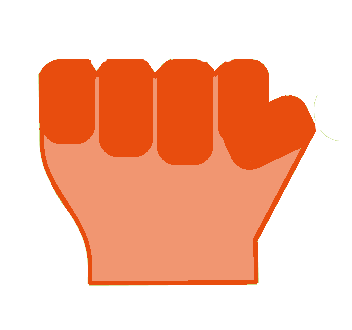
- "Rock" [All fingers are flexed]
- "Scissor" [Forefinger and middle finger are extended and the remaining ones are flexed]

|
|

|
| Paper | Rock | Scissor |
Acquired Data:
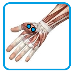
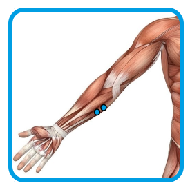
- Electromyography (EMG) | 2 muscles | Adductor pollicis and Flexor digitorum superficialis
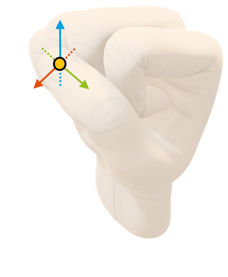
- Accelerometer (ACC) | 1 axis | Sensor parallel to the thumb nail (Z Axis perpendicular)
Protocol/Acquisition Procedure
1 - Placement of EMG electrodes for monitoring muscular activity
1.1 - Placement of electrodes for monitoring muscular activity of
Adductor pollicis
1.2 - Placement of electrodes for monitoring muscular activity of Flexor digitorum superficialis
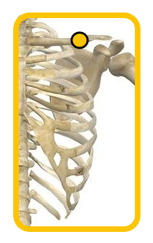
1.3 - Selection of a bone structure away from the active muscles (in our case the clavicle was used)
|
|
|
| Adductor pollicis | Flexor digitorum superficialis | Ground electrode on clavicle |
2 - Fixation of accelerometer to the nail of the thumb
3 - Start of signal acquisition procedure
3.1 - Execute OpenSignals software
3.2 - Access the "Device Configuration" screen
At this stage it should be activated the three needed channels ( CH1 Flexor digitorum superficialis | CH2 Adductor policis | CH3 Accelerometer axis Z).In order to fulfill the Nyquist Theorem statement, a sampling rate of at least 1000 Hz should be selected for ensuring a correct acquisition of EMG data without losing any informational content.
For a more detailed information about the configuration procedure there is a Jupyter Notebook entitled "Signal Acquisition [OpenSignals]"
3.3 - Start signal acquisition/recording procedure, taking into consideration the experimental protocol described below
It is all ready for collecting some training data !!!
The experimental protocol is divided into 4 parts (1/available class). For each class we gathered EMG and ACC data for 5 times (trials).
So, at the final we have 20 training examples (5/available class).
Experimental Protocol
- Collection of training examples for class 0 ["No Action"]
- Hand was kept relaxed during 5 seconds
- Stop acquisition after 5 seconds
- Store file with a formal name ([class number]_[trial number].txt > 0_[trial number].txt )
- Repetition of the procedure A for 5 times
- Collection of training examples for class 1 ["Paper"]
- Immediately after starting the acquisition, volunteer should make a coordinate extension of hand fingers
- Stop acquisition after 5 seconds
- Store file with a formal name ([class number]_[trial number].txt > 1_[trial number].txt )
- Repetition of the procedure A and B for 5 times
- Collection of training examples for class 2 ["Rock"]
- Immediately after starting the acquisition, volunteer should fold all fingers of the monitored hand
- Stop acquisition after 5 seconds
- Store file with a formal name ([class number]_[trial number].txt > 2_[trial number].txt )
- Repetition of the procedure A and B for 5 times
- Collection of training examples for class 4 ["Scissor"]
- Immediately after starting the acquisition, volunteer should extend the forefinger and middle finger and fold the remaining fingers of hand
- Stop acquisition after 5 seconds
- Store file with a formal name ([class number]_[trial number].txt > 3_[trial number].txt )
- Repetition of the procedure A and B for 5 times
Graphical Representation of the Acquired Data
One representative trial of each class is presented below !Class "No Action"
Class "Paper"
Class "Rock"
Class "Scissor"
We reach the end of the "Classification Game" first volume. If you are feeling your interest increasing, please jump to the next
volume
![]() .
.
We hope that you have enjoyed this guide.
biosignalsnotebooks
is an environment in continuous expansion, so don"t stop your journey and learn more with the remaining
Notebooks
![]() !
!