Generation of a time axis (conversion of samples into seconds)

Difficulty Level:

All electrophysiological signals, collected by PLUX acquisition systems, are, in its essence, time series.

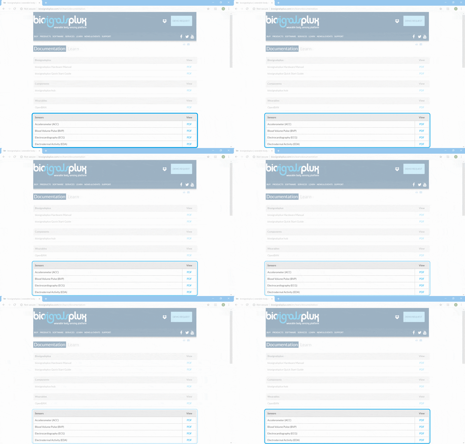
Raw data contained in the generated .txt, .h5 and .edf files consists in samples and each sample value is in a raw value with 8 or 16 bits that needs to be converted to a physical unit by the respective transfer function.

PLUX has examples of conversion rules for each sensor (in separate .pdf files), which may be accessed at "Documentation>>Sensors" section of biosignalsplux website.

Although each file returned by OpenSignals contains a sequence number linked to each sample, giving a notion of "time order" and that can be used as x axis, working with real time units is, in many occasions, more intuitive.

So, in the present Jupyter Notebook is described how to associate a time axis to an acquired signal, taking into consideration the number of acquired samples and the respective sampling rate.

1 - Importation of the needed packages

# Package dedicated to download files remotely
from wget import download

# Package used for loading data from the input text file and for generation of a time axis
from numpy import loadtxt, linspace

# Package used for loading data from the input h5 file
import h5py

# biosignalsnotebooks own package.
import biosignalsnotebooks as bsnb

A - Text Files

A1 - Load of support data inside .txt file (described in a Jupyter Notebook entitled "Load acquired data from .txt file" )

# Download of the text file followed by content loading.
txt_file_url = "https://drive.google.com/uc?export=download&id=1m7E7PnKLfcd4HtOASH6vRmyBbCmIEkLf"
txt_file = download(txt_file_url, out="download_file_name.txt")
txt_file = open(txt_file, "r")

# [Internal code for overwrite file if already exists]
import os
import shutil
txt_file.close()
if os.path.exists("download_file_name.txt"):
    shutil.move(txt_file.name,"download_file_name.txt")
    txt_file = "download_file_name.txt"
txt_file = open(txt_file, "r")

A2 - Load of acquisition samples (in this case from the third column of the text file - list entry 2)

txt_signal = loadtxt(txt_file)[:, 2]

A3 - Determination of the number of acquired samples

# Number of acquired samples
nbr_samples_txt = len(txt_signal)

from sty import fg, rs
print(fg(98,195,238) + "\033[1mNumber of samples (.txt file):\033[0m" + fg.rs + " " + str(nbr_samples_txt))

Number of samples (.txt file): 417150

B - H5 Files

B1 - Load of support data inside .h5 file (described in the Jupyter Notebook entitled "Load acquired data from .h5 file" )

# Download of the .h5 file followed by content loading.
h5_file_url = "https://drive.google.com/uc?export=download&id=1UgOKuOMvHTm3LlQ_e7b6R_qZL5cdL4Rv"
h5_file = download(h5_file_url, out="download_file_name.h5")
h5_object = h5py.File(h5_file)

# [Internal code for overwrite file if already exists]
import os
import shutil
h5_object.close()
if os.path.exists("download_file_name.h5"):
    shutil.move(h5_file,"download_file_name.h5")
    h5_file = "download_file_name.h5"
h5_object = h5py.File(h5_file)

B2 - Load of acquisition samples inside .h5 file

# Device mac-address.
mac_address = list(h5_object.keys())[0]

# Access to signal data acquired by the device identified by "mac_address" in "channel_1".
h5_signal = list(h5_object.get(mac_address).get("raw").get("channel_1"))

B3 - Determination of the number of acquired samples

# Number of acquired samples
nbr_samples_h5 = len(h5_signal)

print(fg(232,77,14) + "\033[1mNumber of samples (.h5 file):\033[0m" + fg.rs + " " + str(nbr_samples_h5))

Number of samples (.h5 file): 417150

As it can be seen, the number of samples is equal for both file types.

print(fg(98,195,238) + "\033[1mNumber of samples (.txt file):\033[0m" + fg.rs + " " + str(nbr_samples_txt))
print(fg(232,77,14) + "\033[1mNumber of samples (.h5 file):\033[0m" + fg.rs + " " + str(nbr_samples_h5))

Number of samples (.txt file): 417150
Number of samples (.h5 file): 417150

So, we can simplify and reduce the number of variables:

nbr_samples = nbr_samples_txt

Like described in the Notebook intro, for generating a time-axis it is needed the number of acquired samples and the sampling rate .

Currently the only unknown parameter is the sampling rate , which can be easily accessed for .txt and .h5 files as described in "Signal Loading - Working with File Header" .

For our acquisition the sampling rate is:

sampling_rate = 1000 # Hz

AB4 - Determination of acquisition time in seconds

# Conversion between sample number and seconds
acq_time = nbr_samples / sampling_rate

print ("Acquisition Time: " + str(acq_time) + " s")

Acquisition Time: 417.15 s

AB5 - Creation of the time axis (between 0 and 417.15 seconds) through linspace function

time_axis = linspace(0, acq_time, nbr_samples)
print ("Time-Axis: \n" + str(time_axis))

Time-Axis: 
[0.00000000e+00 1.00000240e-03 2.00000479e-03 ... 4.17148000e+02
 4.17149000e+02 4.17150000e+02]

AB6 - Plot of the acquired signal (first 10 seconds) with the generated time-axis

bsnb.plot(time_axis[:10*sampling_rate], txt_signal[:10*sampling_rate])

This procedure can be automatically done by generate_time function in conversion module of biosignalsnotebooks package

time_axis_auto = bsnb.generate_time(h5_file_url)

from numpy import array
print ("Time-Axis returned by generateTime function:")
print (array(time_axis_auto))

Time-Axis returned by generateTime function:
[0.00000000e+00 1.00000240e-03 2.00000479e-03 ... 4.17148000e+02
 4.17149000e+02 4.17150000e+02]

Time is a really important "dimension" in our daily lives and particularly on signal processing analysis. Without a time "anchor" like sampling rate it is very difficult to link the acquired digital data with real events.

Concepts like "temporal duration" or "time rate" become meaningless, being more difficult to take adequate conclusions.

However, as can be seen, a researcher in possession of the data to process and a single parameter (sampling rate) can easily generate a time-axis, following the demonstrated procedure.

We hope that you have enjoyed this guide. biosignalsnotebooks is an environment in continuous expansion, so don"t stop your journey and learn more with the remaining Notebooks !

☌ Project Presentation
☌ GitHub Repository
☌ How to install biosignalsnotebooks Python package ?
☌ Signal Library

☌ Notebook Categories
☌ Notebooks by Difficulty
☌ Notebooks by Signal Type
☌ Notebooks by Tag

from biosignalsnotebooks.__notebook_support__ import css_style_apply
css_style_apply()

.................... CSS Style Applied to Jupyter Notebook .........................